Exocomet search

In this tutorial we use nuance to search for exocomet transits on \(\beta\) Pictoris planetary system.

Note

This tutorial requires the lightkurve package to access the data.

In order to run this tutorial on all available CPUs, we set the XLA_FLAGS env variable to

import os
import jax

jax.config.update("jax_enable_x64", True)
os.environ["XLA_FLAGS"] = f"--xla_force_host_platform_device_count={os.cpu_count()}"

Download

We start by downloading the data using the lightkurve package

import lightkurve as lk
import numpy as np
import matplotlib.pyplot as plt

# single sector
lc = lk.search_lightcurve("beta pic", author="SPOC", exptime=120)[5].download()

# masking nans
time = lc.time.to_value("btjd")
flux = lc.pdcsap_flux.to_value().filled(np.nan)
error = lc.flux_err.to_value().filled(np.nan)
mask = np.isnan(flux) | np.isnan(error) | np.isnan(time)

# we only want to analyze the first 3000 points
# mask[time < 1423] = True
time = time[~mask].astype(float)
flux = flux[~mask].astype(float)
error = error[~mask].astype(float)

# normalize
flux_median = np.median(flux)
flux /= flux_median
error /= flux_median

plt.plot(time, flux, c="0.5", label="raw data")
_ = plt.xlim(time.min(), time.min() + 1)

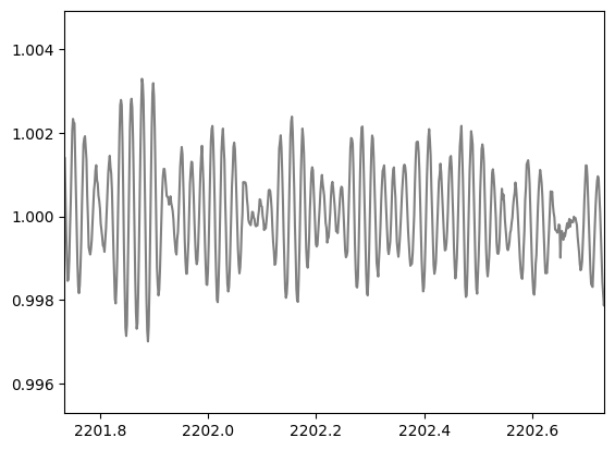
The raw data shows a flux dispersion of about \(10^{-3}\), which is mainly due to \(\delta\) Scuti pulsations in the stellar atmosphere. In order to search for exocomets while modeling this signal, we will define and optimize a Gaussian Process (GP) model of the data.

Gaussian Process

In order to define a GP able to represent the pulsation of the star, let’s find its rotation period using a Lomb-Scargle periodogram

def rotation_period(time, flux):
    """rotation period based on LS periodogram"""
    from astropy.timeseries import LombScargle

    ls = LombScargle(time, flux)
    frequency, power = ls.autopower(
        minimum_frequency=1 / 10, maximum_frequency=1 / 0.01
    )
    period = 1 / frequency[np.argmax(power)]
    return period


period = rotation_period(time, flux)
print(f"P = {period:.3f} days")

P = 0.021 days

We then define the GP kernel as a mixture of two SHO kernels (implemented in nuance.kernels) and representative of a wide range of stellar variability signals.

import jax.numpy as jnp
from nuance.kernels import Rotation
from tinygp import GaussianProcess, kernels

initial_params = {
    "log_period": jnp.log(period),
    "log_Q": jnp.log(100),
    "log_sigma": jnp.log(jnp.std(flux)),
    "log_dQ": jnp.log(100),
    "log_f": jnp.log(2.0),
    "log_jitter": jnp.log(jnp.mean(error)),
}


def build_gp(params, time, mean=0.0):
    jitter2 = jnp.exp(2 * params["log_jitter"])

    kernel = Rotation(
        jnp.exp(params["log_sigma"]),
        jnp.exp(params["log_period"]),
        jnp.exp(params["log_Q"]),
        jnp.exp(params["log_dQ"]),
        jnp.exp(params["log_f"]),
    )
    return GaussianProcess(kernel, time, diag=jitter2, mean=mean)

And proceed to its optimization

from nuance.utils import minimize
from nuance.core import gp_model

mu, nll = gp_model(time, flux, build_gp)

# optimization
gp_params = minimize(nll, initial_params, ["log_sigma", "log_period"])
gp_params = minimize(nll, gp_params)

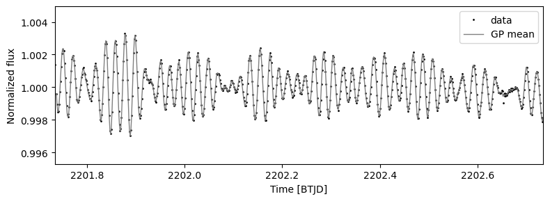
Let’s see the fitted light curve

Show code cell source Hide code cell source

import matplotlib.pyplot as plt

plt.figure(figsize=(8, 3))
plt.plot(time, flux, ".", c="k", ms=2, label="data")

gp_mean = mu(gp_params)
split_idxs = [
    0,
    *np.flatnonzero(np.diff(time) > 10 / 60 / 24),
    len(time),
]

_ = True
for i in range(len(split_idxs) - 1):
    x = time[split_idxs[i] + 1 : split_idxs[i + 1]]
    y = gp_mean[split_idxs[i] + 1 : split_idxs[i + 1]]
    plt.plot(x, y, "0.5", label="GP mean" if _ else None, lw=1)
    _ = False

plt.xlabel("Time [BTJD]")
plt.ylabel("Normalized flux")
plt.legend()
plt.tight_layout()
_ = plt.xlim(time.min(), time.min() + 1)

gp = build_gp(gp_params, time)

Exocomet search

All the above is the GP preparation, now is time to actually search the light curve.

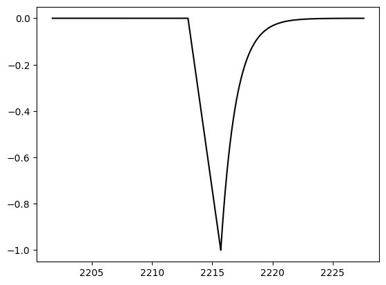
Here we employ a model template of an exocomet transit with varying durations. We note that this model is purely empirical.

import jax.numpy as jnp
import matplotlib.pyplot as plt


def exocomet(time, t0, duration, period=None, n=3):
    flat = jnp.zeros_like(time)
    left = -(time - (t0 - duration / n)) / (duration / n)
    right = -jnp.exp(-2 / duration * (time - t0 - duration / n)) ** 2
    triangle = jnp.maximum(left, right)
    mask = time >= t0 - duration / n
    signal = jnp.where(mask, triangle, flat)
    return signal / jnp.max(jnp.array([-jnp.min(signal), 1]))


_ = plt.plot(time, exocomet(time, np.mean(time), 5), c="k")

Linear search

Let’s compute the SNR of single exocomet transit events as our detection metric

from nuance import core
from tqdm import tqdm

durations = np.linspace(1 / 24, 1.5, 20)

# vmap over durations
snr_function = jax.jit(
    jax.vmap(
        jax.jit(core.snr(time, flux, gp=gp, model=exocomet)), in_axes=(None, 0, None)
    )
)
snrs = np.array([snr_function(t0, durations, None) for t0 in tqdm(time)])
snr = snrs.max(1)

100%|██████████| 17458/17458 [02:16<00:00, 128.24it/s]

from scipy.signal import find_peaks

plt.figure(figsize=(8, 6))

min_snr = 6
ms = 3
ax = plt.subplot(3, 3, (1, 3))
ax.plot(time, snr, "-", c="k")
ax.axhline(min_snr, c="k", alpha=0.2)
peaks, _ = find_peaks(snr, height=min_snr, distance=0.5 / np.diff(time).mean())
peaks = peaks[np.argsort(snr[peaks])[::-1]][0:3]
peaks = peaks[np.argsort(time[peaks])]
plt.plot(time[peaks], snr[peaks] + 4, "v", c="k", ms=ms)
# remove x axis and spine
ax.spines["bottom"].set_visible(False)
ax.spines["top"].set_visible(False)
ax.spines["right"].set_visible(False)
ax.set_xticks([])
ax.set_yticks([0, min_snr, 12, 20])
ax.set_xlim(time.min(), time.max())
ax.set_ylabel("SNR")

signals = []
for peak in peaks:
    t0 = time[peak]
    j = np.argmax(snrs[peak])
    D = durations[j]
    signals.append(core.separate_models(time, flux, gp=gp, model=exocomet)(t0, D))

signals = np.array(signals)

plt.subplot(3, 3, (4, 6))
plt.plot(time, flux, ".", c="0.8", ms=1, label="raw data")
plt.plot(time, np.min(signals[:, 1], axis=0) + 1.0, "k", label="max-SNR signals")
plt.xlim(time.min(), time.max())
plt.ylabel("relative flux")
plt.legend(loc="upper right")

for i, peak in enumerate(peaks):
    ax = plt.subplot(3, 3, 7 + i)
    linear, astro, noise = signals[i]
    plt.plot(time, flux, ".", c="0.85", ms=ms, label="raw" if i == 2 else None)
    plt.plot(
        time,
        flux - noise,
        ".",
        c="0.5",
        ms=ms,
        label="detrened" if i == 2 else None,
    )
    plt.plot(time, astro + 1, c="k", label="model" if i == 2 else None)
    xmin, xmax = time[peak] + 2 * np.array([-1, 1]) * durations[np.argmax(snrs[peak])]
    plt.xlim(xmin, xmax)
    plt.ylim(0.999, 1.001)
    if i != 0:
        ax.set_yticklabels([])
    else:
        ax.set_ylabel("relative flux")
    if i == 1:
        ax.set_xlabel("time [BTJD]")
    if i == 2:
        ax.legend(loc="upper right")

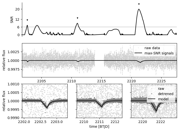
We can now plot the first three highest SNR events

These were found by Lecavelier des Etangs et al. 2022, who first removed the pulsations of the star using a Fourrier decomposition of the light curve (detrending one harmonic at a time). This was enabled by the high quality factor of the \(\delta\) Scuti variations, and would have been challenging in the case of a pseudo-periodic stellar variability.