Single transit search#
In this notebook, we use nuance to search for a single transit.
Generating the data#
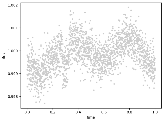
Let’s generate some data first, of a unique planetary transit lost in a smooth stellar variability signal
import numpy as np
from tinygp import kernels, GaussianProcess
from nuance import core

depth = 1e-3
error = 0.5e-3
time = np.linspace(0, 1, 2000)
transit_prams = {"epoch": 0.3, "duration": 0.05, "period": 10}
transit_model = depth * core.transit(time, **transit_prams)
kernel = kernels.quasisep.SHO(10.0, 200.0, 0.005)
gp = GaussianProcess(kernel, time, diag=error**2)

flux = transit_model + gp.sample(jax.random.PRNGKey(0)) + 1.0
import matplotlib.pyplot as plt

ax = plt.subplot(111, xlabel="time", ylabel="flux")
plt.plot(time, flux, ".", c="0.8")
plt.tight_layout()
The linear search#
We can now look for single transit events by performing the linear_search over all times (considered as potential transit epochs) and on a wide range of durations.
from nuance.linear_search import linear_search

epochs = time.copy()
durations = np.linspace(0.01, 0.2, 15)

ls_function = linear_search(time, flux, gp=gp)
lls, depths, vars = ls_function(epochs, durations)
Important
nuance relies on tinygp to manipulate Gaussian processes. Although gp in the previous cell is already a tinygp.GaussianProcess instance (from the simulated data), in practice one has to build their own.
To have an idea of where the potential candidates might be, let’s plot the unique transit log-likelihood computed during the linear search.
plt.subplot(211)
plt.plot(time, flux, ".", c="0.8")
plt.ylabel("flux")

plt.subplot(212)
plt.imshow(
    lls.T,
    aspect="auto",
    origin="lower",
    extent=[time.min(), time.max(), durations.min(), durations.max()],
)
plt.ylabel("durations")
plt.xlabel("time")

plt.tight_layout()
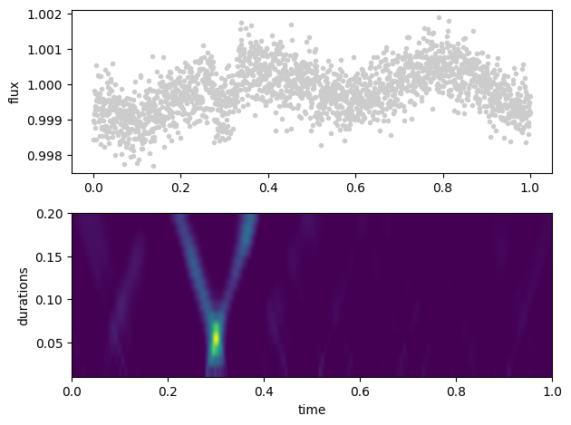
We clearly identify a transit candidate
i, duration_i = np.unravel_index(np.argmax(lls), lls.shape)
t0, D = epochs[i], durations[duration_i]

print("\n".join([f"{n}: {v:.3f}" for n, v in zip(["epoch", "duration"], [t0, D])]))
epoch: 0.301
duration: 0.051
that we can plot thanks to its parameters
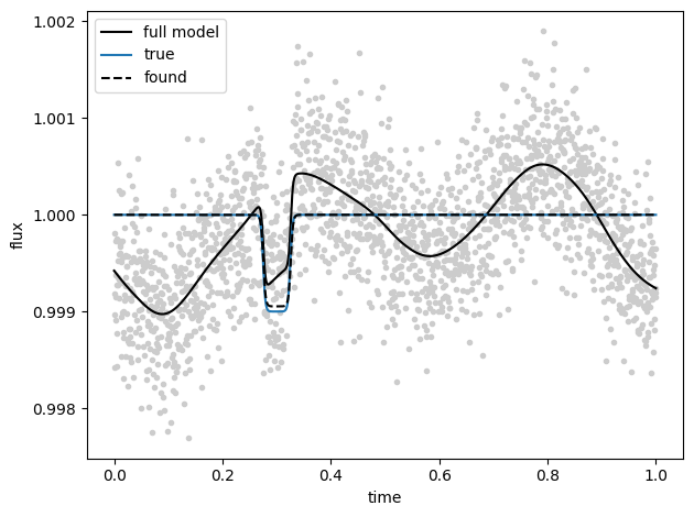
Which is the one injected in the simulated dataset